Inspired by this tweet from Scott Weingart, I thought I'd demonstrate some ways to convert a skyline image into a waveform! (An opportunity for some basic sonification.)
To be clear, we'll work with a basic 2D skyline where all we have are heights. It might be interesting to think of each building as its own wavelet and mix them together in sequence, or use some techniques from the Sonification Handbook, but the roof contours of individual buildings are a little harder to obtain, so let's stick to a 2D outline for now.
Some basic image processing with scikit-image will allow us to extract the skyline itself. There are then two simple ways to turn it into sound: directly converting the skyline into an amplitude envelope, or treating the image as a frequency-domain representation and using an inverse FFT.
Method 1: Amplitude envelope
In this case, we create a waveform that has the same envelope as the skyline image. This means that the resulting sound's loudness is proportional to the buildings' heights.
%matplotlib inline
import numpy as np
import matplotlib.pyplot as plt

from skimage import feature, filters, io, morphology
from scipy import ndimage
import librosa
import librosa.display # must be imported separately

from IPython.display import Audio, Image
# Load the Boston skyline image https://commons.wikimedia.org/wiki/File:Boston_Twilight_Panorama_3.jpg
# by Wikimedia Commons user Fcb981 https://commons.wikimedia.org/wiki/User:Fcb981
# CC BY-SA 3.0

skyline_url = "https://upload.wikimedia.org/wikipedia/commons/6/67/Boston_Twilight_Panorama_3.jpg"
skyline = io.imread(skyline_url)
Image(url=skyline_url)
# Cropping and thresholding to capture just the outline.

lx, ly, _ = skyline.shape
skyline_cropped = skyline[: -lx // 4, :, 2]

threshold = filters.threshold_isodata(skyline_cropped)
thresholded = skyline_cropped > threshold

outline = np.argmin(thresholded, axis=0)
outline = skyline_cropped.shape[0] - outline

thresholded = thresholded[::-1, :]

fig, axes = plt.subplots()
axes.plot(outline, color='r')
axes.imshow(thresholded, cmap=plt.cm.gray, origin='lower')
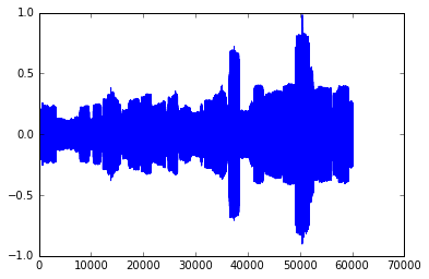
Armed with the outline as a series of y-values, we can create the corresponding amplitude envelope in the range [0.0, 1.0] and multiply it by white noise. (We stretch out the envelope so that the evolution of the sound can be heard).
envelope = outline / outline.max()
stretched_envelope = envelope.repeat(10)

# generate white noise in the range [-1.0, 1.0)
waveform = ((np.random.rand(*stretched_envelope.shape) - 0.5) * 2)

# impose envelope on noise
waveform *= stretched_envelope

fig, axes = plt.subplots()
axes.plot(waveform)
Audio(waveform, rate=22050)
Sounds, well, like noise.
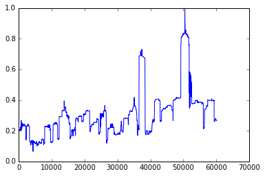
It's also possible to simply play back the envelope itself (although due to the DC offset it isn't good for your speakers). Since sound is essentially variation in pressure, and the pressure doesn't change widely enough in the envelope, this doesn't sound like much.
fig, axes = plt.subplots()
axes.plot(stretched_envelope)
Audio(stretched_envelope, rate=22050)
Method 2: Inverse FFT
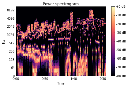
The other common way of turning images into sound is to use an inverse FFT. This treates the image's y-axis as frequency, meaning that the highest pitches correspond to the contours of the roofs.
NB: The resulting audio is much louder than the above, and quite shrill.
skyline_ifft = librosa.istft(thresholded)

D = librosa.stft(skyline_ifft)

fig, axes = plt.subplots()
plt.sca(axes)

librosa.display.specshow(librosa.amplitude_to_db(D, ref=np.max),
                         y_axis='log', x_axis='time')
plt.title('Power spectrogram')
plt.colorbar(format='%+2.0f dB')
plt.tight_layout()
Audio(skyline_ifft, rate=22050)
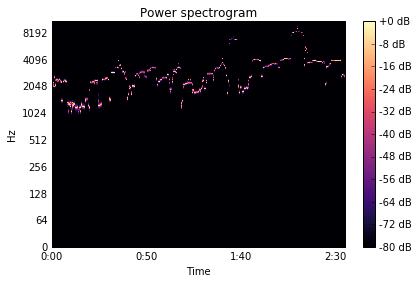
It's possible to sonify just the tops of the buildings, rather than the whole image, but it sounds somewhat dull (and again a bit loud).
outline_2d = np.zeros(thresholded.shape)

for i, y in enumerate(outline):
    outline_2d[y, i] = 1.0

outline_ifft = librosa.istft(outline_2d)

D = librosa.stft(outline_ifft)

fig, axes = plt.subplots()
plt.sca(axes)

librosa.display.specshow(librosa.amplitude_to_db(D, ref=np.max),
                         y_axis='log', x_axis='time')
plt.title('Power spectrogram')
plt.colorbar(format='%+2.0f dB')
plt.tight_layout()
Audio(outline_ifft, rate=22050)
These very basic conversions aren't very pleasant to the ear, but they only scratch the surface of what is possible.
See the original gist if you want to play with the code.
If you have any interest in how to convey data using sound, I suggest you check out the Sonification Handbook's examples; for example, the model-based sonification offers some interesting possibilities.


